Whether are concerns are related to landslides, pollution, wetland habitat, weather, engineering, or water resources, one of the most common work flows in GIS is the estimation of watersheds and associated hydrologicla flow features over a landscape. These kinds of models can get very complex, and are often ground-truthed in the field. However, this is not a hydrology class. Here, I will introduce the basic building blocks of stream and catchment delineation in GIS, with a few notes about external resources that may help you. Key questions we want answered when performing hydrolgoy in QGIS are:
-
- Where is water flowing?
- How much of it is flowing?
- Where are the channels that carry the water?
- What area of the landscape drains to a particualr point?
Even more than other methods, hydrology in QGIS has at least 3 different toolkits that can be applied to solve the same problems. Which toolkit you apply is a matter of experience and preference. For most typical GIS applications, the SAGA toolbox & Raster Calcualtor are all you neeed. However, if you wish to do dynamic or statistical models in hydrology, the best options are WhiteBox and PCRaster.
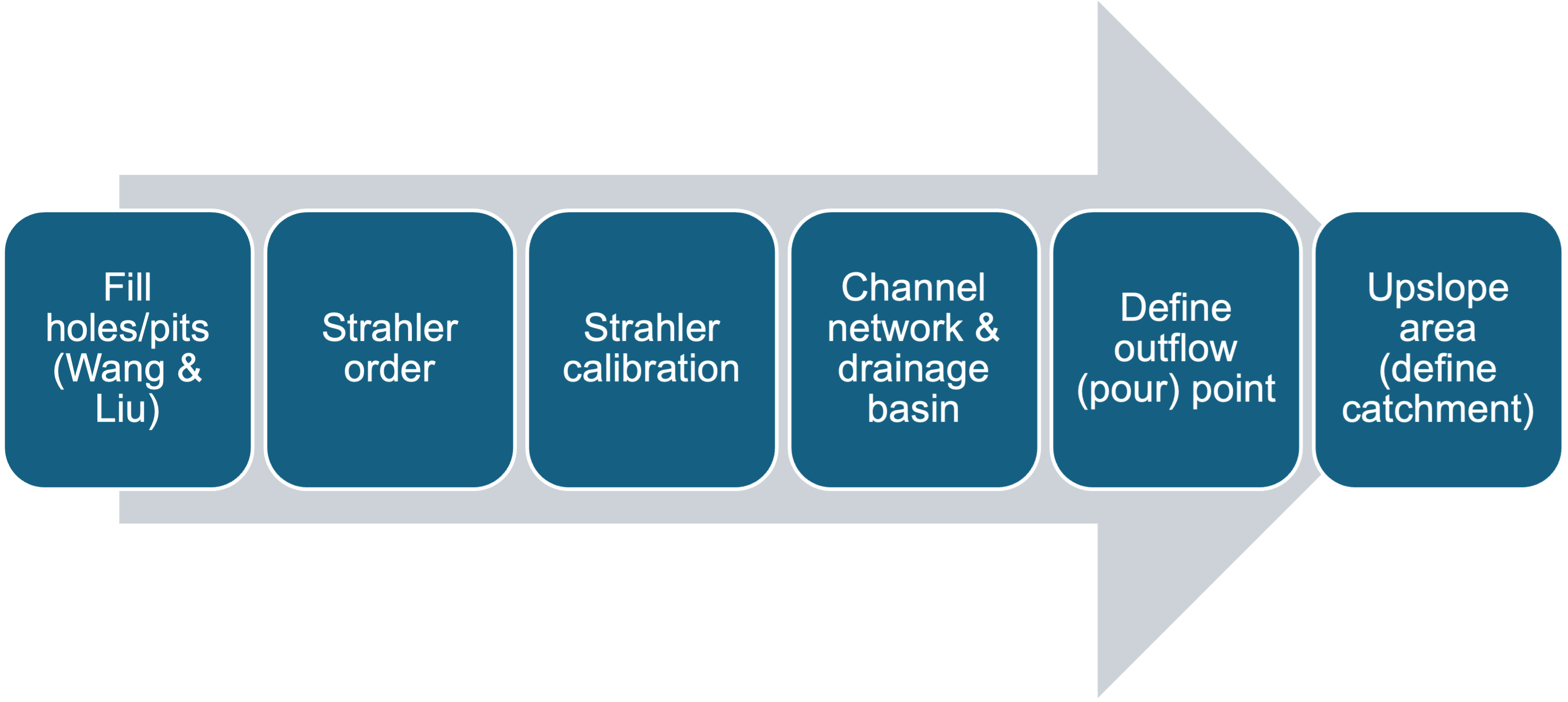
The basic workflow in QGIS follows this flow diagram, with some exceptions:
Input
In most hydrological applications, your main input is going to be a DTM raster file. You may also have raster files that represent precipitation, temperature, soil cover, bedrock geology, vegetation, etc….all features that affect water’s behavior in the landscape.
Fill holes (Wang & Liu)
In order to determine where water is going to flow, we need to remove artifacts from the DTM that would cause the water to pool. These sinks or peaks are usually artifacts of the layer’s resolution, not real data features. So We can use the Fill holes (Wang & Liu) algorithm, which either raises or lowers surroundign cells to elvel everything out:


(NOTE: obviously in nature, siuch sinks exist; but without more sophisticated tools, we aren’t able to use the simple logic of the algorithms mentioned beloe without getting rid of these sinks).
Strahler order calculation & calibration
Streams have been found to approximate a mathematical concept called the Strahler order, where lower-order bracnhes combine to feed yet larger branches, and so-on, and so-forth. Higher order streams carry more water, and above a 6th-10th order, approximate large streams or rivers.
Strahler order presents a problem for us – we need it as an input for later work, but we can;t take every stream from lllow through hgih order, without making the analysis slow and cumbersome. So before moving on, the Strahler order output needs to be thresholded or calibrated; this involves you the user exploring the DTM, and determining which streams contribute the most to the hdyrological feature you are interested in.
***you must document why you chose a particualr threshld!!***

Channel network & Drainage basin
This tool will take the DTM, and your Strahler threshold you determined from the previus step, and output a range of hydrological outputs. The msot important ones are the estimated channels (where does water collect as it flows?) and the catchment areas (also called watersheds). In SAGA, these can be outputted as either raster or vector file formats.
NOTE: If you have a vector or raster layer with reported, measured location of existing chanels, you can use the tool Burn stream network into DEM prior to any of these steps; this will ensure the actual stream area is the lowest elevation point in the DTM; in turn, this will make the flow direction and flow accumulation more accurate.
Define outflow (pour) point
At this stage, you often want to know where a particular downstream point collects water from in the surrounding landscape. Say you wanted to know whether pollution from an abandoned iron mine upstream is affecting the city of Richmond; you’d need to pick the entrance of the James river into Richmond city limits as your outflow or pour point, to then know whether the upsteam drainage from the mine is polluting city waters. In QGIS, you do this using the Coordinate Capture plugin tool, and then define your Outflow point using appropriate SAGA tools.

Upslope area
FInally, to determine your watershed or catchment basin, you fed the coordinates of your outflow point into the Upslope area tool, as well as your filled DTM layer (no sinks). The result will be a raster layer, with value 1 = catchment basiin; value 0 = study area not draining to your outflow point.
Once completed, you now have a map and measurements of the hydrologicla properties of your study area. Further analysis will allow ou to estimate flow rate, water accumulation, flood potential, and even landslide risk.
Helpful video resources
This video contains a short and succinct summary of the steps needed to accomplish basic hydrological analysis in QGIS:
This is a thorough walkthrough of watershed delineation, with live examples. I believe this sues the PCRaster plugin:
Older SAGA version of the above example; mroe relevant for basic hydrological applications:
More detailed look at PCRaster applied to hydrology:
A workflow using the open source Whitebox plugin for hydrology: